From Chapter 5.4 Probability:
A number from 0 to 1 that represents the likelihood of an event occurring is referred to
as the event’s probability. A probability of 0 means that the event is certain not to occur,
and a probability of 1 means that the event is certain to occur. In this section, we will
see that integration is a useful tool for calculating some probabilities.
So this is an earlier chapter than the chapter I took notes on from before. Let’s see: I took notes on chapter 10.3 Discrete Probability Distributions. Weird that I’m now going back and taking notes/doing stuff on what sounds like the basics of probability.
I know this is a calculus text but so far I’ve avoided having to do any integration. I wonder if that trend will continue.
There are two types of probability, experimental and theoretical.
Experimental - based on actual events, you flip a coin a bunch of times, you get tails 52 out of 100 times, you then say the probability is 52/100
Theoretical - based on thinking/reasoning, you reason that since the two sides of a coin seem the same when you flip it it should have a 50% chance of lending on either side.
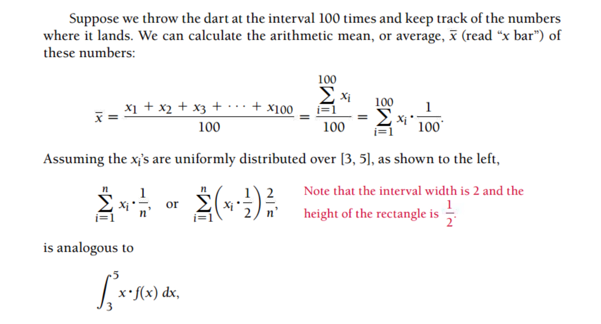
Suppose that we throw a dart at a number line in such a way that it always lands in the
interval [3, 5]. Let x be the number where the dart lands. There is an infinite number
of possibilities for x. Note that x can be observed (or measured) repeatedly and its
possible values comprise an interval of real numbers. Such a variable is an example of
a continuous random variable.
Continuous Random Variable -
its continuous, since their is no break in the values it can hold between 3 and 5. it can hold any and all values between their. the values just continue(?) from one point to another
its random, since it can take on any value in an interval
its variable, well x is defined here as the variable that takes on the differing values as we throw the dart at the number line
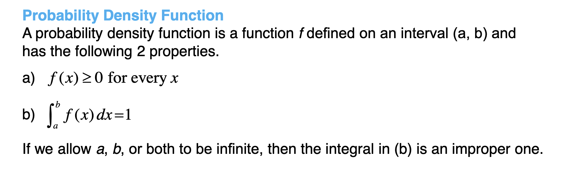
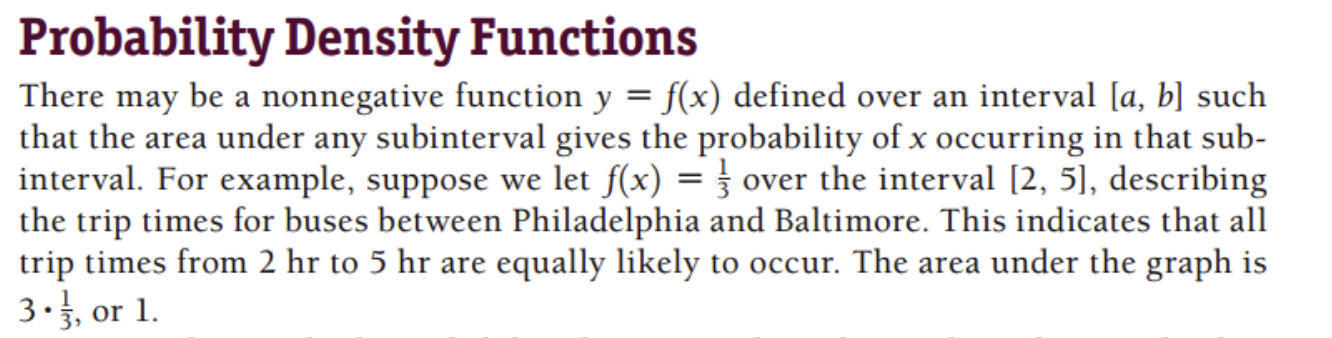
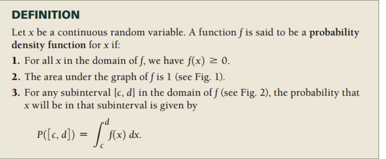
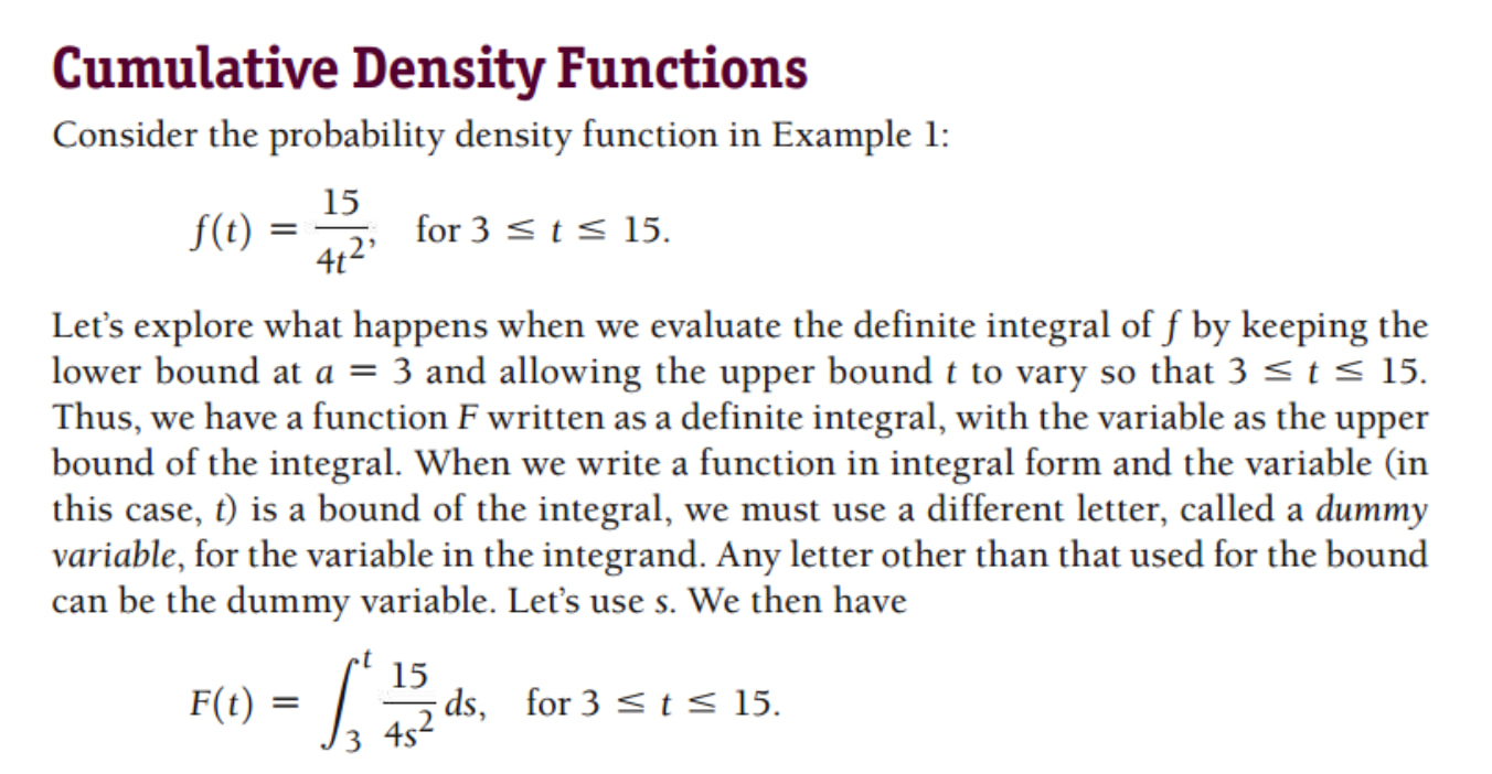
So previously I did probability mass functions. Now I’m doing density functions. Ok.
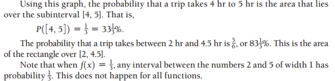
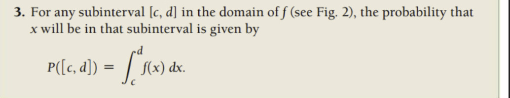
ok so we may be able to take the area of a subinterval which will give us the probability of x occurring in that sub-interval. ok.
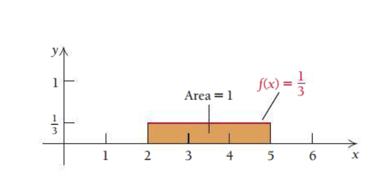
i’m a bit confused on how it explained it, but looking at the picture of the graph it makes sense i think:
So the function here is y/f(x) = 1/3 ? And I guess since probability is defined to be from 0 to 1. You divide that 1 into three parts or something.
that makes sense from 3 to 4 it would be 33%
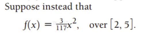
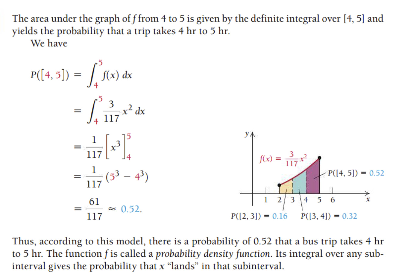
Looking at the next steps seems like this will involve integration. I’m going to try and integrate this:
ok so it looks like i got the integration part right, but i did the wrong thing it seems. doing the integral from 2 to 5 gave me 1.
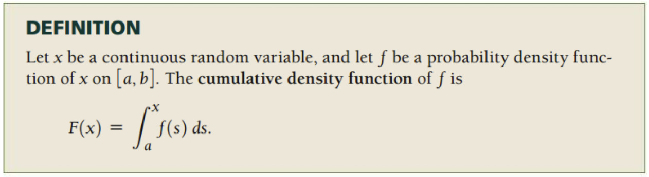
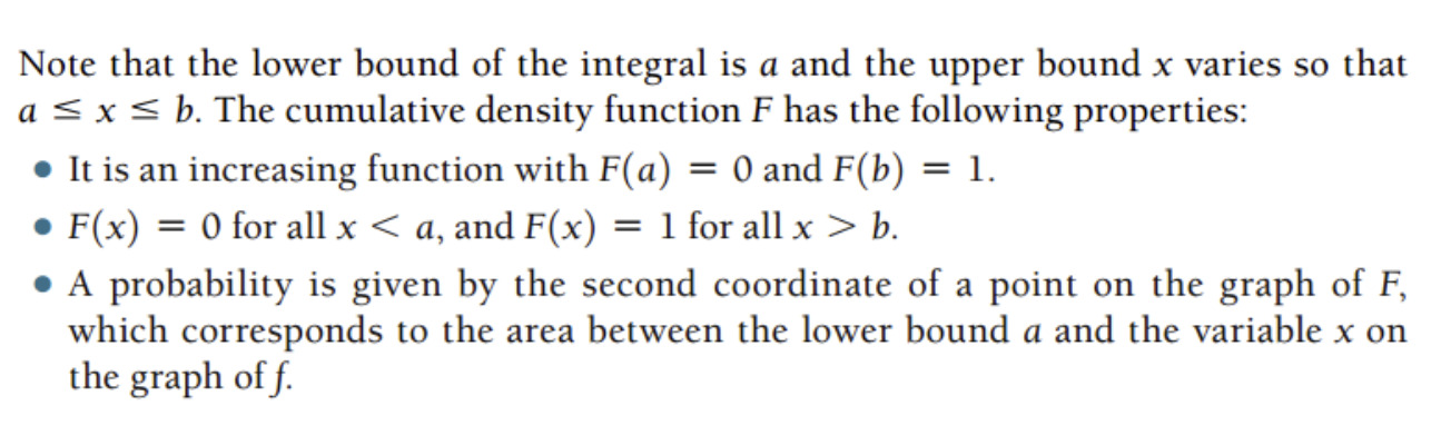
1.) all outputs are positive
2.) the values all add up to 1
3.) that really doesn’t seem like a definition
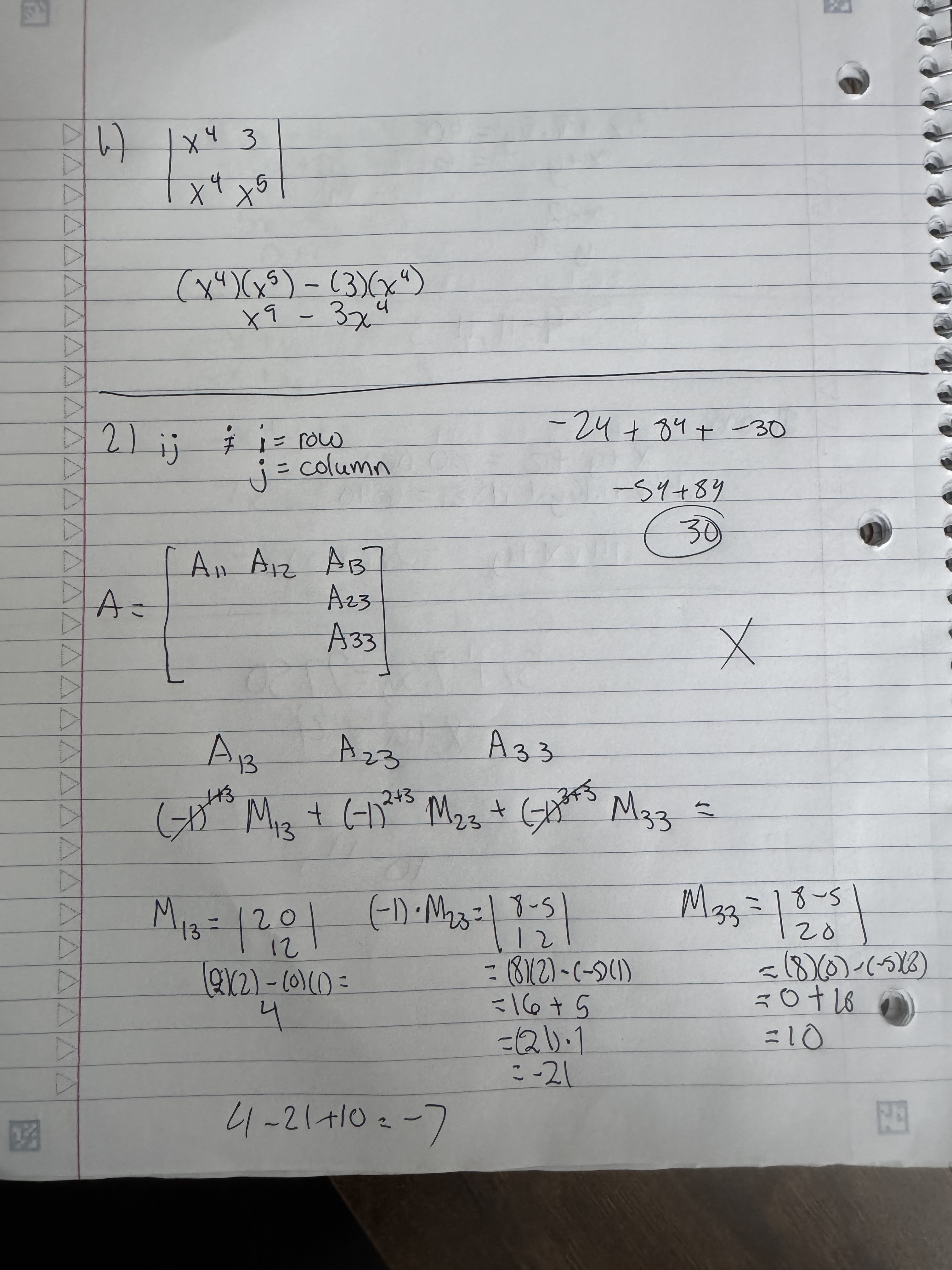
Some homework:
Hmm. I’m only going to share one problem here because all of the problems for this homework were of the same kind.
Question is kind of long so I hid it
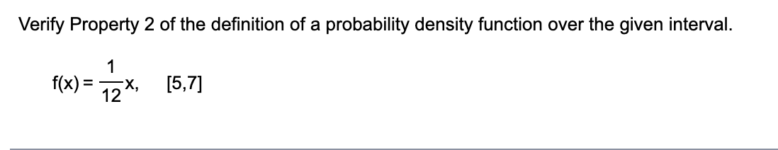
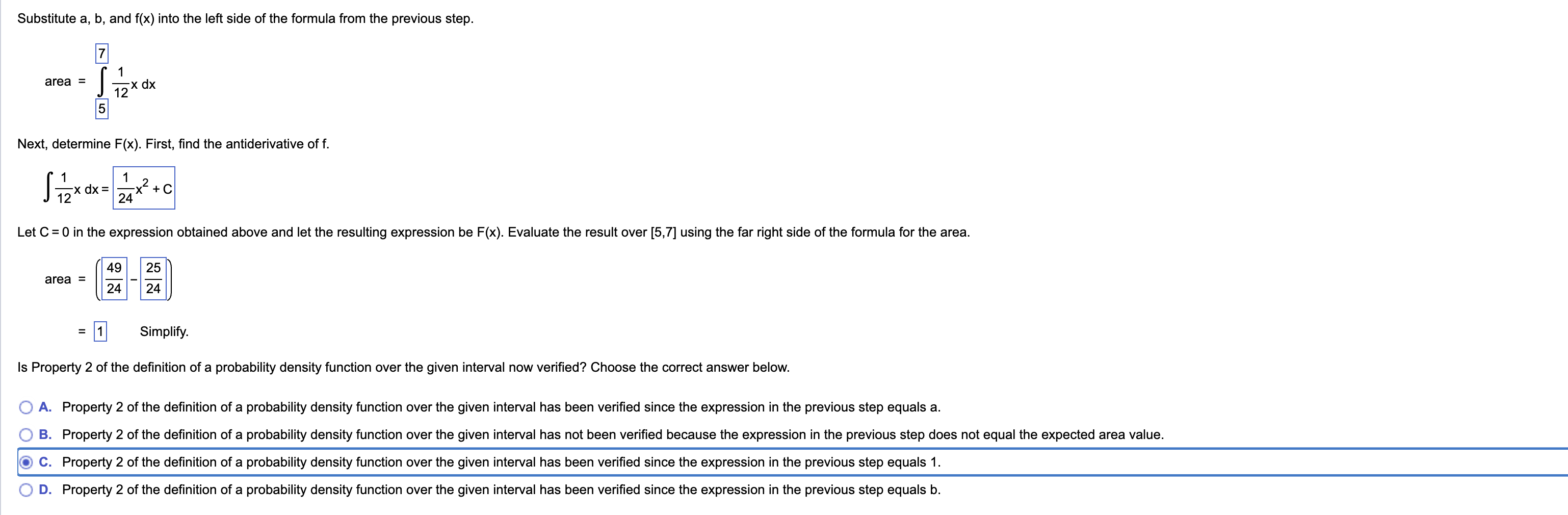
All the questions (5 of them) ask about verifying property 2.
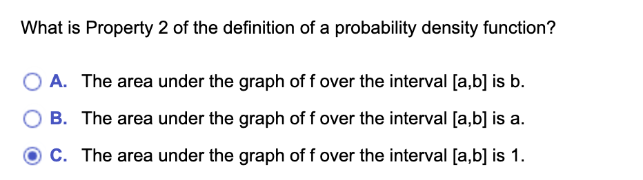
All the questions ask what is property 2 and its the same answer every time
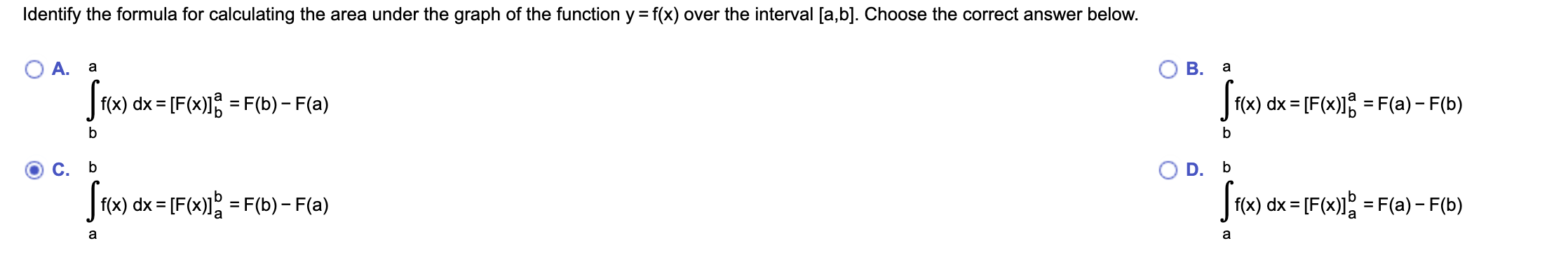
they all ask about the formula for evaluating integrals and its the same every time
they all evaluate out to 1 and the answer to the last question is always that it follows the definition because they always evaluate to 1